

Demystifying What Quantum Computing Can(not!) Do, Part I
Demystifying What Quantum Computing Can(not!) Do, Part I
What computational complexity theory tells us about the power and limits of quantum computers


Papers:
[0] Noisy intermediate-scale quantum algorithms, Bhatari et al. (2022)
[1] The Limits of Quantum, Aaronson (2008)
Unlike my prior three posts, we’re going to take a different tack in this one — instead of summarizing a paper, I’d like to take a topic and pull it apart, using papers as references.
The popular science literature is littered with very poor descriptions of what quantum computers can do. From claims of “Quantum will solve all our problems” to “Quantum is blindingly-fast compared to classical”, lots of misconceptions abound.
This post gives you information to have a realistic perspective on the matter. It will do so by looking at the question of “What can a quantum computer do?” through the rigorous lens of computational complexity theory.
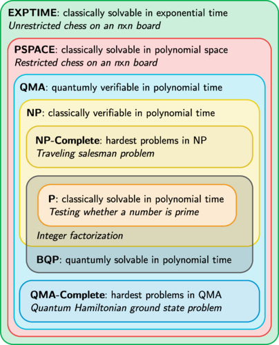
By the time you finish this article, you will understand what Fig 1 is telling you about the power of quantum computers. This figure highlights some of the main classes of problems which are discussed when talking about the power of quantum computing.
As a side note, writing this post is amusing to me. Back in my freshman year at Caltech, I took a computer science class under Professor Chris Umans (CS 21: Decidability and Tractability). It didn’t go very well (but not because of the professor!). I hadn’t had any CS exposure before, so jumping off into the deep end of computational complexity theory was a tad hard. I muddled my way through it, and developed enough background to not be so intimidated by complexity theory. Thanks, Professor Umans!
Key take-aways: quantum computing and complexity theory
Computational complexity theory puts on a rigorous and sound footing what it means for a problem to be “easy” or “hard” for a classical or quantum computer.
Examples exist of problems which are provably easy for quantum computers to solve, but which we suspect will be hard for classical ones. Factoring integers is an example.
There are some problems of practical importance in optimization which we do not think will be easy for quantum computers. Finding provably-optimal routes is an example.
There are well-defined and known limits on the power of quantum computers — not all problems are easy for them.
Before we get started, three small points:
Complexity classes are defined with respect to some model of computation. For classical computers, this model is called a “Turing machine”. It turns out there is a quantum generalization called — appropriately enough — a “quantum Turing machine”, introduced by physicist David Deutsch in 1985. In what follows, when the words “classical computer” or “quantum computer” are used, what I mean is “the corresponding model of computation”.
The word “problem” here means “A collection of problem instances, where each instance is specified by a bitstring of a given length.”. For example, the “factoring problem” would refer to the general problem of factoring integers, not the specific task of factoring a given one.
When computer science researchers began formalizing the notions of the time or space resources required by a Turing machine to solve a problem, they settled on a particular notion of what solving a problem “efficiently” means. Namely, a problem can be solved efficiently if the amount of resources scales polynomially with the size of the bitstring specifying the problem instance. If that bitstring is of size n, then as long as the resources scale at worst as n^a for some value of a, the problem is said to be efficiently solvable.
With those points out of the way, let’s dive in.
Classical Complexity Classes: P and NP
Before getting to quantum, let’s start with something more familiar; namely, classical computers.
The Complexity Class P
Our starting point in Fig 1 is the complexity class P, which stands for “Polynomial Time”. Problems in this complexity class have efficient classical algorithms (i.e., the resources scale polynomially with the problem instance size). That is, given a problem instance, generating a solution using a classical computer is efficient. Examples of problems in P that would be familiar to use include addition, multiplication, and division. Other problems which are also in P, but perhaps less familiar, include linear programming, and checking whether a number is prime. (If the last one is not obvious, that’s OK — this was first established only in 2002!)
Problems in P are considered to be “easy”, because of how computer scientists defined the idea of “hard”. Whether or not the runtime of a given algorithm for solving a problem in P is practical or not is a different point. So you could run into a situation where, given a problem instance, the scaling of the algorithm is so bad that solving that instance would take longer than the known age of the universe, but as long as that scaling is polynomial, then the algorithm is considered “efficient”.
With respect to quantum computing, a reason to go after creating new quantum algorithms to tackle problems known to be in P is to devise new algorithms which have a more favorable scaling.
The Complexity Class NP
The class P consists of problems for which generating solutions is efficient. The next class we turn to in Fig 1, NP, consists of problems for which verifying a proposed solution is efficient. NP stands for “Non-Deterministic Polynomial Time”, because NP was originally formulated as the class of problems efficiently solvable using a non-deterministic Turing machine. For our purposes, it suffices to know that an entirely equivalent formulation is “The set of problems whose solutions are efficiently checkable. Note that NP says nothing about whether generating a solution is efficient. A famous open question in computer science is whether P and NP are actually the same complexity class.
The class NP gets talked about quite a bit in the context of quantum computing, often wrongly. In particular, within NP there is the set of so-called “NP-complete” problems, which are problems representative of the hardness of the NP class. These problems include 3-SAT, the traveling salesman problem, graph coloring, and a whole host of others. NP-complete problems can be thought of as the hardest problems in NP, because any problem in NP can be efficiently transformed into an NP-complete problem. This means any improvements in algorithms for NP-complete problems automatically are very important.
Here’s the catch when it comes to quantum: if you ever hear someone say “Quantum computers will efficiently solve NP-complete problems.”, tell them to stop, because they are — at least as of the time of this post — wrong. People erroneously think that because of the phenomenon of quantum superposition, quantum computers could evaluate all possible solutions to an NP-complete problem simultaneously, and thereby return an answer. This is not true — we do not expect that the class of problems efficiently solvable using a quantum computer (more on that below) includes NP-complete problems.
If you ever hear someone say “Quantum computers will efficiently solve NP-complete problems.”, tell them to stop, because they are — at least as of the time of this post — wrong.
That said, there is evidence quantum computers can efficiently solve some problems in NP (but again, not NP-complete ones!). Consider the problem of factoring integers: I give you an integer N, and you tell me what prime numbers I have to multiply together to make N. This problem is in NP, because if someone proposes a set of prime factors for N, it’s very easy to check whether they are: just multiply the proposed prime factors together to see if the result equals N. So you can efficiently check whether a proposed solution is in fact one.
Now we know — from Shor’s factoring algorithm — that the problem of factoring integers is efficiently solvable using a quantum computer. So we know there is at least 1 problem in NP which is efficiently solvable using a quantum computer.
But what about others?
Quantum Complexity Classes: BQP and QMA
The two complexity classes most relevant for quantum computers are BQP and QMA. These are — in a well-defined sense — the quantum versions of P and NP, respectively. But there are some modifications needed to account for the fact that the output of a quantum computation is usually probabilistic (that is, multiple runs of the same algorithm, with the same inputs, yield different outputs). For this reason, unlike the classical complexity classes discussed above, we need some notion of randomness — and the possibility an algorithm might fail — built in.
The complexity class BQP (“Bounded-Error Quantum Polynomial Time”) is the set of problems solvable in polynomial time with quantum computers, with high probability (in particular, 2/3). That is, the runtime of the algorithm is efficient (in the computer science sense of “is polynomial”), and the algorithm has to output the correct answer at least 2/3 of the time.
We saw an example of a problem in BQP (factoring), and there are many others. (See for example the Quantum Algorithms Zoo.) In addition, it is believed (but not proven) that BQP extends outside of NP — that is, there are problems for which solutions can be efficiently generated by quantum computers, but those solutions cannot be efficiently verified by classical ones. An unambiguous resolution to that question would be of huge importance to the fields of computer science and quantum computing.
BQP is the set of problems whose solutions can be efficiently generated by quantum computers. The class QMA (“Quantum Merlin Arthur”) is the set of problems whose proposed solutions can be efficiently checked with quantum computers. And just like how there exists NP-complete problems (e.g., traveling salesman), there also exist QMA-complete ones. For example, if I give you a quantum-mechanical description of a physical system (such as a molecule), where that description has certain properties, then the task of telling me “This is the lowest possible energy configuration this system could attain.” is QMA-complete. (That’s the “Quantum Hamiltonian ground state estimation problem” in Fig 1.)
The relationship between BQP and QMA is currently unknown, though in analogy with P and NP, it’s suspected that QMA is bigger than BQP. This implies quantum computers could efficiently check some solution to a problem, but couldn’t efficiently create it. (Where would that solution come from? I’m not sure.)
Beyond QMA
The world of computational complexity theory is quite rich, as Fig 1 shows. There are 2 more complexity classes to briefly discuss, because they show us there exist problems which are well beyond those which quantum computers can efficiently solve. This cuts to the heart of the bad narratives you see out there; namely, “Quantum will solve everything”. It’s just not the case — quantum computers will be really, really good at some problems, and not others. That’s OK.
Quantum computers will be really, really good at some problems, & not others. That’s OK.
The other 2 classes, PSPACE and EXPTIME, are really big. PSPACE is the set of problems which can be solved using a polynomial amount of space (but not time). Here, “space” can be thought of as meaning “memory allocated”. And EXPTIME is — as you might guess from the name — the set of problems which can be solved using an exponential amount of time.
It is known that BQP cannot extend outside PSPACE (paper ref [1] above). And it’s widely believed PSPACE is not the same as EXPTIME. This tells us that the power of quantum computers is circumscribed, not unbounded.
Wrap-Up
In this post, we took a tour of computational complexity theory to get a handle on what, rigorously, are the capabilities and limits of what quantum computers can do. We saw that quantum computation does extend the set of problems which are efficiently solvable beyond that which can be done classically. However, it is in no way a panacea to make all problems efficiently solvable.
We also saw that the exact boundaries between classical and quantum computation are not yet fully clear — while there are hunches and intuitions, unambiguous proofs1 showing, for example, P and BQP are separate classes remain elusive.
This post covered the topic of the power of quantum computation through a very rigorous lens. In part II, I will discuss how to make all this theory practical when it comes to looking at addressing real-world problems with quantum.
Additional Resources
If you want to know more about this topic, here are a few things to read:
For the expert reader, here I mean “proofs which do not use oracles”.